Web-based Reanalyses Intercomparison Tools (WRIT)
WRIT Tools
Atmosphere
Ocean
Product Descriptions
Atmospheric or Oceanic Monthly/Seasonal Plotting Page:
Allows users to make maps and vertical
cross-sections from various reanalyses. Statistics include means, anomalies and climatologies.
Users can also difference the various reanalyses for all three types of statistics (for any
overlapping date in the reanalyses). Composites (averaging multiple dates) are also available.
Atmospheric or Oceanic Monthly Time-Series Extractor/Analyzer:
Extracts time-series at specified latitude/longitude
or latitude/longitude ranges and either plots the time-series, time-series differences, and scatter plots.
Various statistics are returned in addition to numeric values of the time-series plotted.
Ability to plot and compare climate index time-series such as
the PNA or Niño3.4 or upload your own.
Atmospheric or Oceanic Monthly Correlation Plotter:
Calculates correlations (and regressions) of the
reanalysis and observational dataset with supplied atmospheric/ocean indices or user uploaded
time-series. Users can plot correlations at different lead/lags. They can also create vertical
cross-section correlation plots.
Atmospheric Trajectory Generator:
Allows users to plot forward and backward air
trajectories from different reanalyses (currently NCEP R1, NCEP R2, and 20CR, and ERA-Interim).
Users can plot the trajectories of one or more levels on a single plot. The output is plotted on
a map and is available as netCDF and as KMZ files suitable for Google Earth.
Atmospheric Distribution Analyzer:
Allows users to plot and compare the distributions of
daily data during a season from different sources including different reanalyses (currently
NCEP R1 and 20CR) and observed data. Users can see where data values have fallen historically
and can see how different distribution assumptions impact the tails of the distribution.
Atmospheric or OceanVertical Profiles:
Allows users to plot different vertical products from
reanalyses including skew-T, variable/height, time by height, and vertical transects (daily data) for the atmosphere and depth by latitude/longitude/time plots for monthly ocean datasets.
Atmospheric Hovmollers:
Allows users to make plots of daily and subdaily time by latitude or time by longitude for different reanalysis datasets. Statistics include means and anomalies.
Posters/Talks
- Ocean WRIT Talk at the fall 2020 AGU meeting.
- Ocean WRIT: preliminary PPT
Publication
- Smith C. A., G. P. Compo and D. K. Hooper (November 2014): Web-Based Reanalysis Intercomparison Tools (WRIT) for Analysis and Comparison of Reanalyses and Other Datasets. Bull. Am. Meteorol. Soc., 95 (11), 1671-1678. doi:10.1175/BAMS-D-13-00192.1
Future WRIT Tool Enhancements
- Lead/Lag time-series relationships
- Spatial correlations comparing different reanalyses
Future Atmospheric WRIT Products
We are exploring the feasibility of various tools. The features we hope to have are:
- Daily time scale composites atmospheric reanalyses.
- Sub-Daily composite atmospheric reanalyses
- Creation and comparison of index time-series such as the PNA from the various atmospheric reanalyses
Future Ocean WRIT Products
- Comparison of buoy and profile data
Background
- Reanalyses.org: A wiki for advancing reanalyses. Users can find information about reanalyses (atmosphere, ocean, land), how to access and plot data, reanalyses observations, diagnostics, and more. Members can post information and ask questions of the reanalysis community.
- Caveats. Also see specific tool information.
- Smith C. A., G. P. Compo and D. K. Hooper (November 2014): Web-Based Reanalysis Intercomparison Tools (WRIT) for Analysis and Comparison of Reanalyses and Other Datasets. Bull. Am. Meteorol. Soc., 95 (11), 1671-1678. doi:10.1175/BAMS-D-13-00192.1
Datasets
There are two types of gridded datasets in the PSL WRIT tools pages. They are atmosphere and ocean reanalysis and gridded observations/analysis. Each web tool uses different sets of datasets depending on what it is plotting/analyzing, our storage, server, and memory resources. There is a link from each page to the datasets used.- Monthly ATMOS WRIT mapping page datasets.
- Monthly ATMOS WRIT time-series page datasets.
- Monthly OCEAN WRIT datasets.
- List of index time-series for ATMOS WRIT (PNA, ENSO, NP,...)
- List of index time-series for OCEAN WRIT
Ocean WRIT How to Guide
- Create a map of a single variable for one season?
- Change the plotting options for a map of a single variable?
- Examine anomalies for latest climate normal (1981-2010 long term mean)?
- Examine anomalies using a custom year range for the long term mean?
- Compare variables over different decades?
- Compare climate phenomena such as ENSO?
- Compare climate phenomena with 2 phases (e.g. El Niño and La Niña)?
- Plot latitude by depth over a longitude range?
- Plot longitude by depth over a latitude range?
- Create a map of time-series correlated with variable?
- Look at index time-series leading a variable?
- Plot a trend?
- Use your own time-series with the correlation tool?
- Plot a vertical cross-section correlation plot?
- Extract a time-series from a latitude/longitude extent of a dataset?
- Compare the same time-series from 2 datasets?
- Plot a pregenerated time-series?
- Create a scatter plot?
- Extract a time-series for use in correlation or time-series page?
- Use your own time-series (1 or both)?
- Create a land or ocean only time-series?
- Perform wavelet analysis on a time-series?
- Plot the autocorrelation of a time-series?
- Create a "heatmap" plot (year by month)?
- Sort a time-series?
- Find period of extreme values ?
| Extract a time-series from a latitude/longitude extent of a dataset?
Select a dataset (NOAA OI SST) and variable (Skin T/SST). Select a rectangular region (Nino 3: -5 to 5, 210 to 270). Select Anomaly. | 
|
| Compare the same time-series from 2 datasets?
Select two datasets (SODA3-JRA55, NCEP GODAS) and u current at 5m. Select Anomaly. Select Nino3 region (-5 to 5, 210E to 270E). Choose key in bottom right. | 
|
| Plot a pregenerated time-series?
Select "Pregenerated Time-series" for dataset. Select "Battery Park Tidal gauge". Plot 1900 to 2020. Select X range 1900 to 2025. | 
|
| Create a scatter plot?
Compare precipitation and salinity over the tropical Pacific. Choose dataset 1 SODA3-JRA55 salinity, 5m. Choose dataset 2 GPCP V2.3 precipitation. Select scatterplot. Enter -4 to 4; 200E to 200E. | 
|
| Extract a time-series for use in correlation or time-series page?
Select Dataset NCEP GODAS. Select variable net heat flux. Enter area 15N; 300E. On page with plot, select link to "Data Table". Save page as text in browser. You can upload to PSL web-tools including the ocean WRIT time-series or correlation tools. | 
|
| Use your own time-series (1 or both)?
From the extract a time-series above, upload it to anonymous ftp following instructions. Select pregenerated time-series and then user upload. Type your title and then the file name ("/Public/incoming/timeseries/yourname"). Select "NH ice extent" from pregenerated time-series. Select season as August to August. | 
|
| Create a land or ocean only time-series?
Select SLP and the JRA-55 dataset. Enter -30 to 30, 0 to 360. Select ocean only. Select Time-series as plot type | 
|
| Perform Wavelet Analysis?
Select Nino 3.4 from pregenerated list of time-series. Use years 1870 to 2019 (need full years of data; no missing). Select plot wavelet | 
|
| Create an autocorrelation plot?
Select the NOAA/PSL PDO (pregenerated time-series). Set time to 1892-2019. Select cross/auto correlation as plot type. | 
|
| Create an autocorrelation plot?
Select the NOAA/PSL Global Temperature NASA (pregenerated time-series). Set time to 1880-2020. Select Heatmap as plot type. | 
|
| Sort a time-series (month by month)?
Select the Nino3.4 Index (HadISST). Plot time-series. Use 1980-2022. Select sort by month. Results have a link to check. | 
|
| Return Extreme Ocean Temperature periods (El Nino) in the Central Tropical Pacific?
Select the NOAA/PSL Nino3.4 Index from the HadISST (pregenerated time-series). Set time to 1870-2022. Select Return Extreme Periods. Minimum Length 11 months. Percentile values >=90%. A list will be returned. | 
|
- Create a temperature profile from a reanalysis?
- Create anomaly profiles from 6 datasets and plot the spread?
- Create the climatological profiles of salinity from 5 different datasets?
- Create a depth transect of a variable from a reanalysis dataset?
- Create an anomalous depth transect of a variable from a reanalysis dataset?
- Create a time by depth plot of a variable at a grid box?
- Create a time by depth anomaly plot at a grid box?
- Plot a Temperature-Salinity Diagram?
- Plot a Temperature-Salinity Climatology Diagram?
